Tolcap enables Designers to predict the process capability of parts even before prototype samples are produced.
Tolcap predicts Cpk - but what is Cpk, and is it the most appropriate process capability index to predict?
The simplest process capability index: Cp.

Recall Control Charts. To set up a control chart for a dimension on a part the dimension is measured on a sample batch of the parts.
The mean (average) and standard deviation, or “sigma” (σ) of the measurements are calculated.
The action limits on the Control Chart are then conventionally set at plus and minus three sigma from the mean.
A thought to hold on to through this blog is that there is an assumption here that these limits are appropriate for the chart plotting future measurements:
while the process is in control, sigma is relatively constant.
To measure process capability, an obvious approach was to compare the tolerance spread with the control chart action limits. Cp does just that:
Cp = (Upper Tolerance Limit - Lower Tolerance Limit) / (Upper Action Limit - Lower Action Limit)
= (Upper Tolerance Limit - Lower Tolerance Limit) / 6σ
Process Shift and Cpk
A problem with Cp is that it assumes the mean of the distribution of the parts is at the centre of the tolerance band.
Real life processes don’t behave that way. Consider a couple of examples:
-
Turning & Boring. For each batch or production run, a setter installs and adjusts the cutting tools to produce the required dimension.
There is a limit to the precision the setter can achieve in centring the distribution of the parts around the nominal dimension between the limits.
-
Plastic Injection Moulding. As the tool is used it will wear.
The toolmaker will make the tool with this in mind: splines on the tool that produce grooves in the part will wear away and the grooves in the part will get smaller as the tool wears - and vice versa.
So the toolmaker makes the splines on the tool oversize to start, to maximise tool life.
For these reasons, process capability is measured using the index Cpk
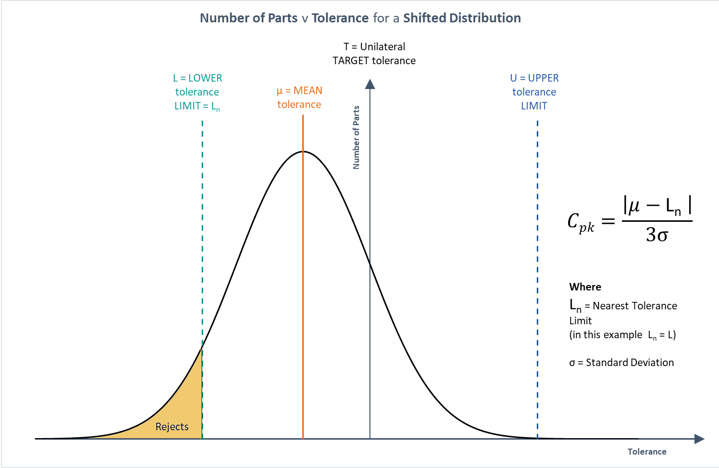
Cpk is calculated by working out which is the nearer limit to the mean of the measured sample.
If the mean is nearer the lower limit (as in the diagram), then
Cpk = (Mean - Lower Tolerance Limit) / 3σ
But if the mean is nearer the Upper Tolerance Limit, then
Cpk = (Upper Tolerance Limit - Mean) / 3σ
Of course if the mean actually does coincide with the centre of the distribution, then Cpk = Cp, but in any other situation Cpk will be smaller than Cp.
The Short Term, The Long Term and Tolcap Predicted Cpk
Let’s look at that last sentence again, thinking carefully about what is being measured.
Yes, if the mean coincides with the centre of the distribution Cpk will be equal to Cp;
but it will be significantly greater than the Cpk measured on the same process when there is a significant mean shift towards either limit.
Think about the examples above:
- Wherever the setter achieves a mean turned dimension above or below nominal, we would expect the spread of parts around that nominal to be similar.
-
Whether early in the tool life or late, we would expect the dimensions of moulded parts around the mean size to be similar
(well, perhaps a little more variable as the tool wears).
As most manufacturing and control chart theory assumes, it is sigma that should be (more or less - within its statistical distribution)
constant if the process is under control.
In consequence, as Cpk is sampled throughout the life of the process it will vary primarily as a consequence of the mean of the samples moving
around the tolerance band, rather than the “spread” of the sample growing or shrinking.
In the case of the moulding Cpk will start small and increase as the tool wears to the nominal size,
then decrease as the tool wears further until it is re-furbished or replaced.
For the turned part Cpk will vary depending on how close the setter got to nominal on that batch.
What is important - as emphasised below - is that the required target Cpk is achieved on any day throughout the life of the process.
For that reason, Tolcap predicts a value of Cpk with a suitable allowance for the offsets that will be measured over the long term.
Sometimes results will be better, they should not be worse.
Equivalent PPM
Look up Cpk versus PPM on the internet and you will invariably find tables quoting twice the value we claim for Tolcap
| Frequently quoted online |
| Process Capability, Cpk |
Rejected parts per million (ppm) |
| 0.33 |
317,300 |
| 0.67 |
45,500 |
| 1 |
2,700 |
| 1.33 |
63 |
| 1.5 |
|
| 1.67 |
0.6 |
| 2 |
0.002 |
| Used by TOLCAP |
| Process Capability, Cpk |
Rejected parts per million (ppm) |
| 0.33 |
161,100 |
| 0.67 |
22,200 |
| 1 |
1,350 |
| 1.33 |
33 |
| 1.5 |
3.4 |
| 1.67 |
0.3 |
| 2 |
< 0.1 |
Why is this?
For a process under control we consider sigma is constant. We have explained that mean shift will vary over time and/or batch to batch.
The variation is process dependent and built into Tolcap predictions,
but for this illustration let us assume we can put a limit on the mean shift equivalent to +/- σ.
(“Six Sigma” assumes +/- 1.5σ, but that is all about detecting a special case,
excessive mean shift * see below.)
Suppose we have specified tolerances to achieve our Tolcap default target Cpk of 1.33.
This means that even with our maximum expected mean shift of +/- σ, the mean size of our part will still be 4σ from the nearest limit.
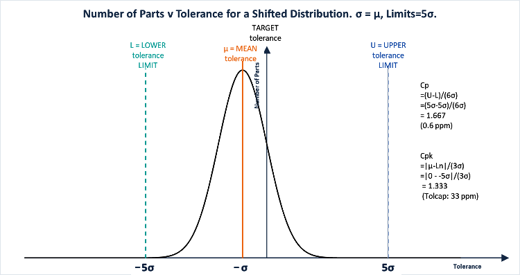
Tolcap's Cpk based PPM prediction reflects a “worst case” scenario.
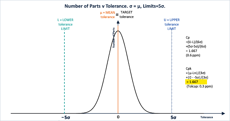
Should the mean coincide with the nominal dimension, we will be 5σ from both limits.
Now in this case we are as likely to see rejects outside the upper limit as outside the lower limit.
The online table, which assumes such a two-sided symmetrical distribution is correct: BUT in this situation,
we have achieved Cpk = Cp = 1.67, and yes, equivalent PPM is 0.6 (!).
Returning to the case where the mean is 4σ from the nearest limit,
we note that the mean is a massive 6σ from the other limit.
So going back to basic single sided standard normal distribution tables, rejects outside the nearer limit contribute 31.5 PPM,
and the contribution from the other limit is negligible at 0.001PPM.
So again, the Tolcap predicted PPM, as the predicted Cpk, is a prediction of the “worst case” on any day.
Cpk or Ppk?
While differentiating short term Cpk measurement from Tolcap’s long term worst case Cpk prediction, this is a good time to review the difference between
Process Capability (Cp, Cpk) and Process Performance (Pp, Ppk).
The formulae for Cpk and Ppk are exactly the same, but the difference is how sigma is calculated.
For Ppk, data is collected for the whole history of the part,
whereas Cpk as we have seen provides a “snapshot” using data from one batch or run of the process.
So as a designer, which would you like to know in advance: Cpk or Ppk?
Well obviously both of them, but Ppk tells you the overall defect rates over the total production, and that can only be history.
Cpk works in the present and tells us whether variation (sigma) is still under control control,
or the process mean has shifted - and there is usually something we can do about that * again see below.
Going back to the Turning and Boring example, if the average dimension is too small, we call the setter back.
In the case of Injection Moulding, we call in the toolmaker to adjust or refurbish the die -
or eventually we find and accept it’s time to replace the tooling. So for this reason, Tolcap predicts Cpk -
what it should not be greater than at any time - rather than Ppk.
Ppk for Ford PPAP
Tolcap acknowledges and responded to the Ford PPAP (Pre-production Part Approval) process.
Ford require suppliers to ensure their parts will prove process capable in series production at Cpk=1.33.
That is why Tolcap’s default acceptable Cpk target is 1.33.
In support of this requirement, Ford requires suppliers to demonstrate Ppk=1.67 on the final pre-production parts manufactured on
the production line process. Ppk?
It is perhaps easy to dodge an explanation by saying that here “P” stands for “Preliminary”,
but is it actually Process Performance they mean?
If the pre-production parts are all from one batch, it makes no difference: the batch is the entire history anyway.
But there may be different batches.
In this case it doesn’t seem unreasonable that the supplier demonstrates the process will consistently be well within limits,
even if the mean has to be re-adjusted, and there is a margin to allow for variation of materials and conditions once full scale
production is under way.
* Why Six Sigma sets a 1.5σ Mean Shift
Nearly everyone who ever went on a Six Sigma course got really confused where that 1.5σ process shift came from.
It came from the original Design for Six Sigma concept that preceded the
DMAIC
quality improvement methodology.
The idea came from semiconductor manufacture in the days when designers would layout a new transistor, process a pilot batch and characterise the device.
The method was to measure sigma for a characteristic of interest, then set the data sheet band for that characteristic at +/- 6σ around the mean.
This allowed 4.5σ to get Cpk = 1.5 allowing 1.5σ for the mean to shift.
That doesn’t reflect any physical natural law that says the mean won’t drift any further:
but note that if the manufacturer maintains a control chart to monitor process shift,
specifically an Xbar-R chart with four samples, the action limit on the Xbar chart comes out at +/- 1.5σ - so they will detect if that happens!
Written by:

Richard Batchelor MA, MBA, CEng, FIEE
Richard is a founding member of the Capra Technology team.